This bio-recipe shows how to find orthologous sequences automatically and how to use them to build a phylogenetic tree of their species.
Orthologous sequences are sequences which belong to different species and have a common homologue exactly in the common ancestor of both species. Paralogous sequences are sequences which were generated by a gene-duplication event without necessarily any speciation. In terms of the following figure, the ellipses represent species and X1, X2 represent genetic sequences. U is the oldest ancestor, which had a single copy of the sequence X1. At some point, between U and its descendant V, a sequence duplication occurred which left two copies of X1. We label the second copy X2. Later, V speciates, that is it has two different descendants, marked A and B. A inherits both sequences X1 and X2 from V. For this example, we have made B inherit only one of the two sequences, in this case X1. X2 was lost or damaged in the evolution from V to B. Now we can say that A[X1] and A[X2] are an example of paralogous sequences.A[X1] and B[X1] are an example of orthologous sequences.More importantly, we consider that A[X2] and B[X1] are not orthologous sequences.
To build phylogenetic trees we need to find orthologous sequences and estimate the amount of evolution between these sequences. Ideally we would like to work on exactly the same protein across all the family that we want to relate. This normally gives better results than using different proteins, as different proteins may be subject to different evolutionary pressures and may give inconsistent estimates of the distances between species. When we can work with the same protein in many species, many inconsistencies disappear.
The most serious danger when evaluating the distance between species through sequences is to use paralogous instead of orthologous sequences. In our picture above, we could have taken B[X1] and A[X2] (which are homologous) and estimate the distance between A and B from them. This would clearly be wrong, as we would be measuring the distance between A, U and B and not A to B alone. Notice, that this mistake could easily happen if A[X1] had not been sequenced (or had been lost in evolution).
The main contribution of this bio-recipe is to explain an algorithm in Darwin which detects orthologous sequences and avoids most of the paralogous ones. Once this is done, we will select a single protein to produce a phylogenetic tree. The selection of a single protein is based on the same ideas used to detect orthology, which is stable pairs. There are several important algorithmic and computational ideas which are developed here.
First we read the SwissProt database and create Dayhoff similarity matrices which will be needed to align sequences.
SwissProt := '~cbrg/DB/SwissProt.Z':
ReadDb(SwissProt);
CreateDayMatrices();
Reading 169638448 characters from file /home/cbrg/DB/SwissProt.Z
Pre-processing input (peptides)
163235 sequences within 163235 entries considered
Peptide file(/home/cbrg/DB/SwissProt.Z(169638448), 163235 entries, 59631787
 aminoacids)
Next we define the desired taxon and collect all the species which can be found in SwissProt (i.e. that have some sequence representation in SwissProt) for that taxon. We print the common name together with the scientific name to make a short table for our own reference. Notice the use of the functions SP_Species which returns a set of species names and SPCommonName which translates a scientific name to a common name, if possible.
taxon := Pinaceae;
species := SP_Species(taxon):
for z in species do
    printf( '%20.20s  %s\n', z, SPCommonName(z) ) od;
taxon := Pinaceae
          Abies alba  Edeltanne
     Abies bracteata  Bristle-cone fir
         Abies firma  Momi fir
       Abies grandis  Grand fir
    Abies holophylla  Neddle fir
     Abies homolepis  Nikko fir
     Abies magnifica  Red fir
      Abies mariesii  Marie's fir
 Abies sachalinensis  Sakhalin fir
      Abies veitchii  Veitch fir
    Cedrus atlantica  Atlas cedar
 . . . . (19 output lines skipped) . . . .
      Pinus pinaster  Maritime pine
         Pinus pinea  Italian stone pine
       Pinus radiata  Monterey pine
       Pinus strobus  Eastern white pine
    Pinus sylvestris  Scots pine
         Pinus taeda  Loblolly pine
    Pinus thunbergii  Green pine
    Pinus virginiana  Virginia pine
Pseudolarix kaempfer  Golden larch
Pseudotsuga menziesi  Douglas-fir
    Tsuga canadensis  Eastern hemlock
  Tsuga heterophylla  Western hemlock
Next we compute the orthologous groups for all the sequences in all the species that we selected. This is done with a single call to Orthologues. We set the printlevel to 2 so that the function prints some information as it works. If there are many sequences involved, this procedure will be very time consuming (as an all against all matching is performed).
printlevel := 2:
orthol_groups := Orthologues( species ):
  1 sequences of Abies alba (Edeltanne) (European silver fir).
  1 sequences of Abies bracteata (Bristle-cone fir).
  2 sequences of Abies firma (Momi fir).
  3 sequences of Abies grandis (Grand fir).
  1 sequences of Abies holophylla (Neddle fir) (Manchurian Fir).
  1 sequences of Abies homolepis (Nikko fir).
  1 sequences of Abies magnifica (Red fir).
  1 sequences of Abies mariesii (Marie's fir).
  1 sequences of Abies sachalinensis (Sakhalin fir).
  1 sequences of Abies veitchii (Veitch fir).
  2 sequences of Cedrus atlantica (Atlas cedar).
  2 sequences of Cedrus deodara (Deodar).
 . . . . (27 output lines skipped) . . . .
 13 sequences of Pinus sylvestris (Scots pine).
  7 sequences of Pinus taeda (Loblolly pine).
  1 sequences of Pinus thunbergii (Green pine) (Japanese black pine), and Pinus contorta (Shore pine) (Lodgepole pine).
  1 sequences of Pinus thunbergii (Green pine) (Japanese black pine), and Pinus koraiensis (Korean pine).
 74 sequences of Pinus thunbergii (Green pine) (Japanese black pine).
  2 sequences of Pinus virginiana (Virginia pine).
  1 sequences of Pseudolarix kaempferi (Golden larch) (Japanese larch).
  1 sequences of Pseudotsuga menziesii (Douglas-fir), and Larix occidentalis (Western larch).
  1 sequences of Pseudotsuga menziesii (Douglas-fir), and Pseudotsuga japonica.
  4 sequences of Pseudotsuga menziesii (Douglas-fir).
  1 sequences of Tsuga canadensis (Eastern hemlock).
  1 sequences of Tsuga heterophylla (Western hemlock).
The parameters given to the function are all the species names that we want to relate. Alternatively, the Orthologues function accepts a sequence. When a sequence is given, it searches the entire database for homologues of the sequence and the orthologous pairs are build from all the matched sequences. The result of the computation is a list of objects called OrthologousGroup each containing one independent group. The groups are ordered by decreasing size, we can look at the smallest one by looking at the last one. The OrthologousGroup contains the list of species, the list of sequences and a matrix of the all-against-all alignments.
orthol_groups[-1];
OrthologousGroup([Pinus strobus, Pinus sylvestris],[
MSVGMGVDLEAFRKSQRADGFASILAIGTANPPNVVDQSTYPDYYFRNTN ..(396).. ETVVLKSIPFP, QVEGV\
VTLSQEDNGPTTVKVRLTGLTPGKHGFHLHEFGDTTNGCMSTGSHFNPKKLTHGAPEDDVRHAGDLGNIVAGSDGVAEA\
TIVDNQIPLSGPDSVIGRALVVHELEDDLGKGGHELSLTTGNAGGRLACGVVGLTPI],[[0, Alignment(Sequence(AC('O65872'))[4..394],Sequence(AC('P30079'))[4..394],4507.2023,DMS[200],3.9236,1.0889,{Local})
], [Alignment(Sequence(AC('O65872'))[4..394],Sequence(AC('P30079'))[4..394],4507.2023,DMS[200],3.9236,1.0889,{Local})
, 0]])
Now we will explain how the orthologous groups are found. The first concept that we define is that of a stable pair of sequences. A stable pair of sequences x1, x2 between two species Spec1 and Spec2 is a pair for which x2 is the highest scoring sequence in Spec2 for x1 and vice versa. The following picture shows this relation.
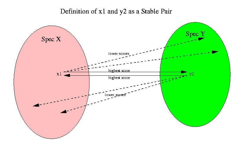
Since we are using Dayhoff matrices for computing the scores, the highest scoring sequences mean the highest level of confidence in homology. By performing and all-against-all alignment for all sequences in every pair of species we find all the stable pairs between pairs of species.
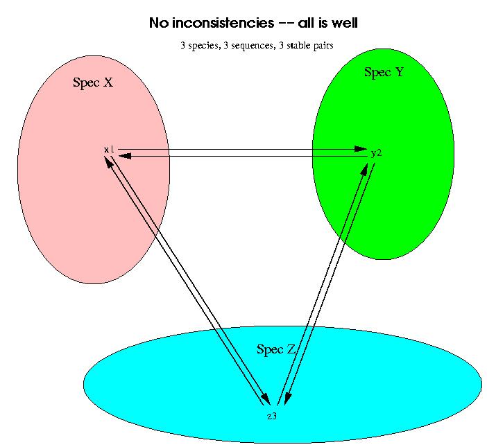
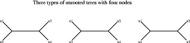
Now we have to weed out the stable pairs which do not correspond to orthology, but to paralogy. This is done through the use of 3 species at a time of which at least two of them have a related stable pair. If all the stable pairs are orthologies, then a triplet of species should look like this:
An example in which a stable pair is not an indicator of orthology but of paralogy is shown in the next figure:
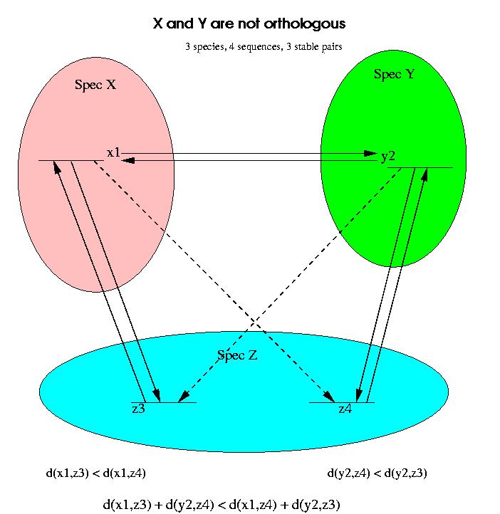
If we compare only the proteins x1 and y2 in Species X and Y, then we might incorrectly assume that the two proteins are orthologs. By comparing with a third genome, it is obvious that this stable pair is invalid and must be broken.
For the analysis of stable pairs we will work with distances instead of similarity scores, but the reasoning is analogous for both measures. We assume that all the alignments involved exist and are reliable (good quality alignments, i.e. score/confidence above certain level). We will now assume that the distance between x1 and z4 is longer than the distance between x1 and z3, i.e.
d(x1,z3) < d(x1,z4)
and similarly the distance between y2 and z3 is longer than the distance between y2 and z4:
d(y2,z4) < d(y2,z3)
These two inequalities are enough to prove that x1 and y2 are not orthologs. If we add these two conditions we obtain:
d(x1,z3) + d(y2,z4) < d(x1,z4) + d(y2,z3)
To prove that x1 and y2 are not orthologs we proceed in two steps.
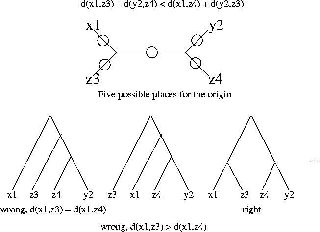
Again we use the above inequalities and the fact that the branches from the root to the leaves must be approximately the same length to discard four of the trees. The third tree is in best agreement with the data.
We have now the proof, the third tree shows that x1 and y2 are not orthologous. The top branch of the tree corresponds to gene duplication (it has z3 and z4 on each side), and hence x1 and y2 arose from gene duplication not speciation.
In simple terms, we use a third species to detect whether pairs are orthologous or paralogous. For this procedure to be successful we need to have at least one species which has been extensively sequenced, and one species which has kept both copies of the original gene duplication. Of course, the more species that are extensively sequenced, even if those sequences end up not participating in the tree, the more credible our orthologs will be. In our example, Green pine is likely to serve as a good witness, as it has a large number of related sequences and stable pairs.
The stable pairs which are not proven paralogous against all the available other species are called verified stable pairs.
The final step is to use the verified stable pairs to make groups. An orthologous group has to have members which are all orthologous with each other. In terms of graphs, if each sequence is viewed as a vertex, and each verified stable pair is viewed as an edge between two sequences (vertices), then an orthologous group is a complete subgraph. In graph theory, a completely connected set of nodes is called a "clique". Finding maximal cliques in a graph is difficult (it is an NP complete problem), but for small problems like we have it is not very time consuming. Darwin implements a very effective clique approximation algorithm which runs in reasonable time. The final step of the Orthologous function is to find the maximal cliques and with each clique form a group. Once that a set of sequences is included in a group, these sequences will not participate in any other clique, that is, any sequence can appear at most once in an orthologous group.
The function Orthologues produces a list of OrthologousGroup data structures. This class is explained in the help file:
?OrthologousGroup
Function BootstrapTree - assign confidence values to internal nodes

Calling Sequence:  BootstrapTree(Ds,labels)
                   BootstrapTree(Ds,labels,nrounds)
                   BootstrapTree(treeofall,bstrees)

Parameters:
  Name        Type              Description
  ---------------------------------------------------------
  Ds          array(matrix)     Distance matrices
  labels      array(anything)   Labels
  nrounds     posint            (optional) number of rounds
  treeofall   Tree              tree of all data
  bstrees     array(Tree)       trees from bootstrapping

Returns:
	Tree
Synopsis:  Computes confidence values to all internal nodes of a tree.  The
  values are integers between 0 and 100, giving the confidence in percents.
  By default, 100 bootstrapping trees from randomly selected distance matrices
  (prob 2/3) are constructed and for each node is counted, in how many
  bootstrapping trees it appears. Each of the input matrices corresponds
  typically to one orthologous group. Alternatively, a tree from all data plus
  a list of trees from bootstapping experiments could be given as arguments.
  The confidence values are stored in the fourth field of the Tree data
  structure and can be displayed using the option InternalNodes =
  ShowBootstrap in the DrawTree function.
See also:  ?DrawTree  ?MinSquareTree  ?PhylogeneticTree  ?Tree


   ------------
We will now display the trees for the two largest orthologous groups, the largest as an unrooted tree, the second largest as a cladogram
DrawTree( orthol_groups[1,Tree], Unrooted,
    Title='Largest phylogenetic tree of the ' . taxon );
ViewPlot();
MinLen not set, using 0.0018474
dimensionless fitting index 131.3
DrawTree( orthol_groups[2,Tree], Cladogram, Legend,
    Title='Second largest phylogenetic tree of the ' . taxon );
ViewPlot();
MinLen not set, using 0.010109
dimensionless fitting index 2.161
The tree fitting index provided by PhylogeneticTree, which is stored in MST_Qual,
MST_Qual;
0.05178019
shows that the quality of the fit is good, (greater than 1 is poor, less than 1 is good). It is just up to the biologist to confirm the quality of the tree.
© 2005 by Gaston Gonnet, Informatik, ETH Zurich
Please cite as:
@techreport{ Gonnet-orthologues,
        author = {Gaston H. Gonnet},
        title = {Finding Orthologous sequences and building a phylogenetic tree},
        month = { March },
        year = {2003},
        number = { 400 },
        howpublished = { Electronic publication },
        copyright = {code under the GNU General Public License},
        institution = {Informatik, ETH, Zurich},
        URL = { http://www.biorecipes.com/Orthologues/code.html }
        }
Last updated on Fri Sep 2 16:41:00 2005 by ghg